METHODs
Tree-ring information was collected from the International Tree-Ring Database (ITRDB) maintained by National Oceanic and Atmospheric Administration (NOAA). The data consist of georeferenced chronology files (.crn) of different tree species, mostly from Argentina and Chile (Figure 4). These chronology files were built by the researcher that uploaded the information and followed a few steps: (1) Ring width measurements are taken in millimeter from tree cores of several trees in a stand (sample and data collection); (2) they are then correlated to each other to accurately assign each growth ring to the correct corresponding growth year (cross-dating); (3) all the width measurements are then transformed to remove age-related trends creating a Ring Width Index file (standardizing); (4) Ring width indexes are then averaged together to produce a mean ring growth index for each year (chronology files). Thus, each chronology represent a stand of forest.
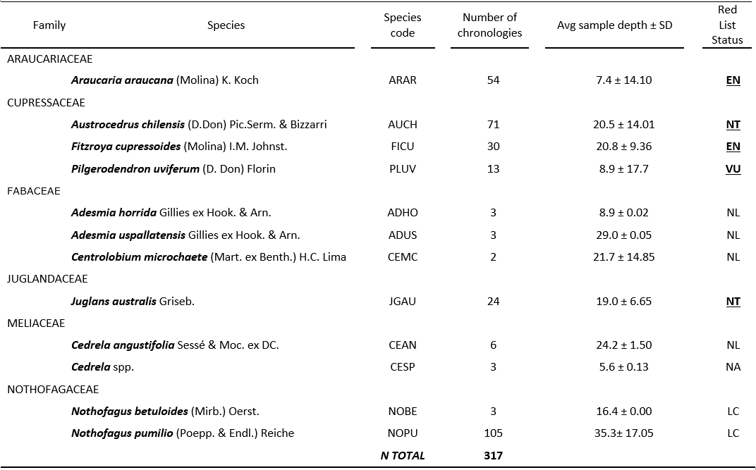
The dataset contained 12 species from six families (Table 1). Two are considered endangered, one vulnerable and one near threat.
The dataset contained 12 species from six families (Table 1). Two are considered endangered, one vulnerable and one near threat.
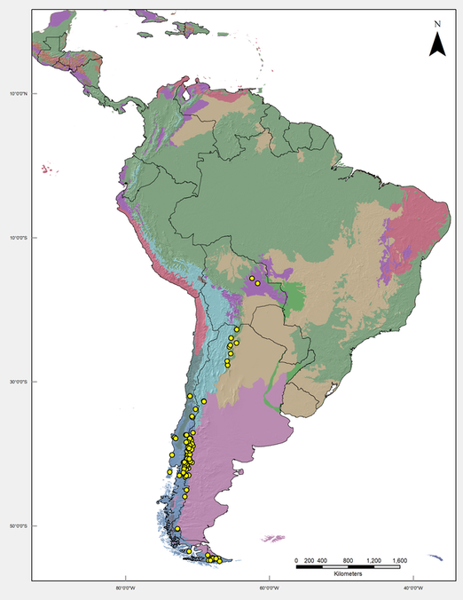
Figure 4. Location of sampled chronologies. Each point represents a forest stand. Points were color coded by species and the different color in the land represent the different ecoregions following (Olson et al. 2001). Black lines represent political borders of the countries in South America.
Table 1. List of species analyzed with their ITRDB codes, number of chronologies analyzed, average sample depth and their respective status in the Red List of Threatened Species of the (IUCN) International Union for Conservation of Nature’s. EN = Endangered, VU = Vulnerable, NT = Near Threat, LC = Least Concern, NL = Not listed in the website and NA = Not applicable. Abbreviations in bold and underlined highlight species with some degree of conservation vulnerability.
The climatic data since 1901 for all the chronologies was acquired from the ClimateSA v1.12 software using the coordinates from each chronology file. This is the earliest available data for climate. The software uses interpolated data generated by Mitchel and Jones (2005) for the years of 1901-2001 which was later updated by Andreas Hamann to include the period of 2001-2013. Over 50 different variables can be obtained. The software is available at http://tinyurl.com/ClimateSA, and was based on methodology described by (Hamann et al. 2013)
To get insight into environmental patterns in the area covered by our data points, we selected eight 8 relevant variables associated with tree growth for a principal component analysis (PCA) (Table 2).
To get insight into environmental patterns in the area covered by our data points, we selected eight 8 relevant variables associated with tree growth for a principal component analysis (PCA) (Table 2).
Table 2. Variable chosen and their respective abbreviations generated with CLIMATE SA Software available at http://tinyurl.com/ClimateSA, based on methodology described by (Hamann et al. 2013).

In the sequence, we applied the clustering algorithm Partition Around Medoids (PAM) (Struyf et al. 1997) using the same variables of the PCA aiming to group data points with similar environmental conditions and reduce complexity of the data. This analysis is based on a dissimilarity matrix that is calculated using Manhattan distances. This algorithm is similar to the clustering algorithm k-means but it is considered to be more robust because the data points are used as anchors for the medoids. Also, this algorithm is embedded with other automated functions to enhance group classification and separation. This algorithm requires you to input the number of cluster. We tested several numbers and chose the one with the least overlap between groups.
To understand what factors drive growth, a response function analysis was performed using the package Treeclim for the software R (Zang and Biondi 2015). For this analysis growth ring information is correlated with monthly average temperature and precipitation. Since the growth on a given year can be influenced by conditions of the previous year growing season, the correlation with climatic variables starts in June of the previous year up to September of the growth year.
In order to test the significance of correlations, the package algorithm follows a bootstrapped procedure (Guiot 1991). Generally, the procedure randomly subsample the observations (years) to create a calibration dataset with the same size of the initial dataset. It does so by omitting some observations and by sampling others more than one time. Then this calibration dataset is then applied to a verification dataset composed by the omitted samples. This procedure is then repeated 50 times yielding 50 regression coefficients 50 multiple correlations and 50 independent verification sets. A mean is calculated out those multiple correlation and significance is tested at 95% confidence interval. If 95% of the coefficients show a positive, or, a negative relationship then the relationship is deemed significant.
Since this analysis is designed to run on a single chronology it does not tell us about geographical patterns. Thus, to investigate the overall occurrence of significant responses in the dataset, all the chronologies with their respective responses for each variable (monthly temperature and precipitation) were plotted in a heat map. They were also subdivided according to cluster (or cluster and species) and ordered by elevation form high to low. Ordering the results allowed further insights into how elevation could be affecting the responses too. Finally, to quantify the responses in a broader geographical scale we calculated the frequency of significant responses within each cluster. This allow us to test the significance of these correlations in a higher scale. For significance testing we followed Chen et al. (2010) work who sets his significance at 25%, that is, if 25% of the chronologies within a region/cluster are found significant then that response is generalized for the whole group.
Lastly, we tested the effect of elevation in the strength of the significance response. This was done by using the coefficient means of the response function analysis of the months that were found to be significant. For example, if temperature of May was found to significantly affect growth, we plotted the mean temperature of May as a function of elevation. In this analysis each chronology is an observation.
