results and discussion
HOW DO CHRONOLOGIES DIFFER IN THEIR RESPONSE TO CLIMATE?
Since the PCA demonstrated considerable overlap among different species, we interpreted that as if they occupy similar ecological ranges. We hypothesized that chronologies under similar climate conditions would respond similarly regardless of what species it is. To explore this hypothesis, the response function of the 317 chronologies were grouped according to the different regions and the frequency of significant results was calculated for each variable, that is, how often do different chronologies respond to the same variables (Figure 9). This analysis showed, overall, that variables of previous year seems not to be frequently related to growth when compared to variables of the same year as growth.
In terms of type of correlation, some chronologies showed opposite responses for the same variable. For instance, in region 4, several variables correlated negatively with growth in some chronologies and positively in others (red bar stacked on green). This demonstrates that the do not respond as similarly as previously thought.
In terms of type of correlation, some chronologies showed opposite responses for the same variable. For instance, in region 4, several variables correlated negatively with growth in some chronologies and positively in others (red bar stacked on green). This demonstrates that the do not respond as similarly as previously thought.
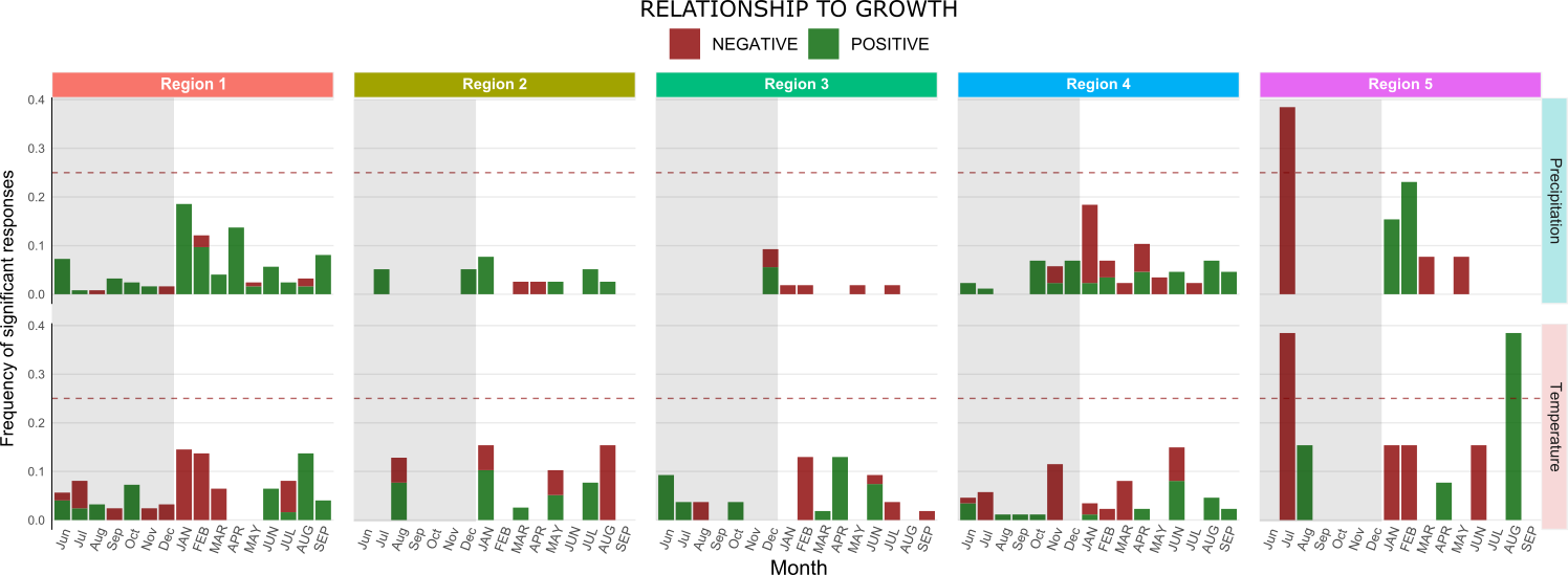
Figure 9. Frequency of significant responses of all 317 chronologies to monthly precipitation and temperature (32 variables total). Variables positively correlated to growth are shown in green and negative correlations in red. Shaded portion of each graph represents correlations to previous year variables and the dashed red line represents the significance threshold at 25%. Bars were stacked for easier representation, however, response is considered significant only if one type of correlation (positive or negative) surpass the 25% frequency threshold. Notice how, in some regions, chronologies showed both positive and negative correlations demonstrating variation in response under similar environmental conditions.
With the exception of region 5, none of the regions had more than 25% of their chronologies consistently demonstrate significant response to any of the 32 variables analyzed. Region 5 has the highest mean annual precipitation of all region (2336mm) with precipitation peaking during the winter in July (300+ mm) and temperatures at its lowest also in July (3.4°C). Negative response to precipitation of previous July could mean that the soil may become to damp for root respiration, what could eventually damage root tissue. As for the negative response to temperature of previous year, this might be related to microorganism’s respiration. If temperature increases, soils aerobic respiration also increases which could speed up oxygen depletion in damp soil, again causing root damage. Such damages would affect tree growth during the next favorable condition. The observed positive response to temperatures of August of current year seems controversial since conditions of this month are very similar to July. We believe that our small sample size (n = 13) may have exaggerated the noise associated with variations in site conditions and species specific response making interpretation and generalizations difficult.
Overall chronologies seems to be generally responding to current year conditions. However clear differences in response among chronologies for the same region demonstrates that chronologies do not respond in the same way under similar conditions. This result led us to investigate if differences observed under the similar climate were species specific.
Overall chronologies seems to be generally responding to current year conditions. However clear differences in response among chronologies for the same region demonstrates that chronologies do not respond in the same way under similar conditions. This result led us to investigate if differences observed under the similar climate were species specific.
For a more reliable interspecific comparison we selected the species with higher number of observations within each region and recalculated the frequency of significant responses accordingly. Our results clearly demonstrate an interspecific variation in response to climate (Figure 10). Within the same region, very different responses are found, with some cases of opposite responses to same variable i.e. temperature of June of current year in Region 4.
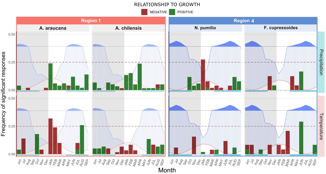
Figure 10. Interspecific comparison of response function analysis for each region. Graphs were overlaid with Walter and Leith diagrams for easier interpretation of results. Notice how different species show different response. A. araucana responds negatively to temperature whereas A. chilensis is indifferent. Similar differences can be observed in region four.
The dataset also provided insights into intraspecific variations in response to climate. The species N. pumulio occurs under different climates of region 3 and 4 and shows considerable variations between sites (Figure 11). In region 4 it demonstrates a negative response to precipitation of January of current year, whereas chronologies from region 3 showed no significant responses to any of the variables. This could be partially explained by to the lower variation in temperature and precipitation throughout the year in region 3, which denotes more steady conditions.
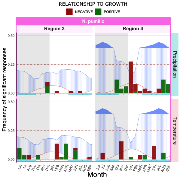
Figure 11. Intraspecific comparison of response function analysis for Nothofagus pumilio. Graphs were overlaid with Walter and Leith diagrams for easier interpretation of results. Notice how the same species shows a different response according to climate. Overall, N. pumilio from region 3 does show a significant response to any of the variables whereas in region 4 its growth was negatively correlated with precipitation of January of current year, which coincides with driest month of the year.
In summary, response to climate in the evaluated dataset depends on a combination of inter and intraspecific variations. Management action as well as any future prediction should take into account how individual species perform under each of climate that it is subjected to.
WHAT ARE THE LIMITING FACTORS FOR TREE GROWTH IN SOUTH AMERICA?
As we seen the limiting factors depend on species and climate together. In Figure 12 it is possible to observe a summary of the limiting factors we found in this work.
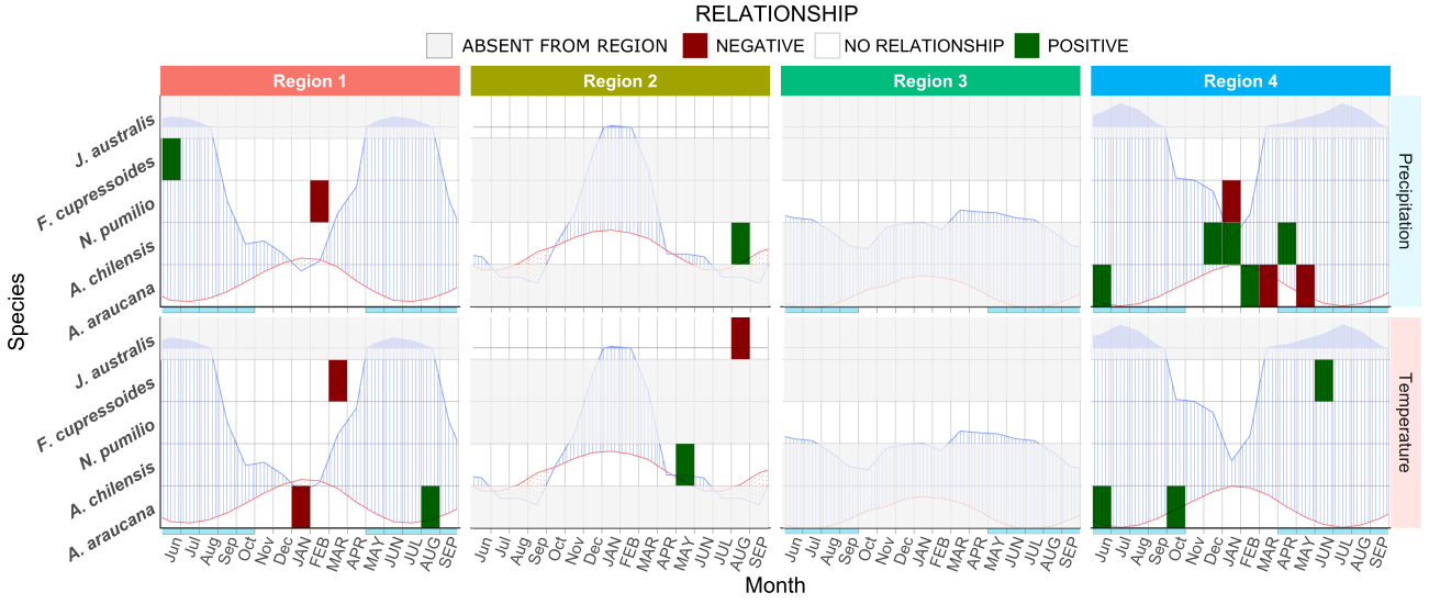
Figure 12. Summary showing the significant correlations found for the different regions according to species. Climate diagrams were overlaid for easier interpretation of the results. Grey stripes mean that the species does not occur in that region.
As a final analysis into the factors that affect tree growth, we investigated how elevation affected the responses. Since higher elevation have generally less precipitation and lower temperatures we hypothesized that elevation could affect responses. When investigating the frequency significant responses at the chronology level we found that at higher elevations the frequency of significant responses increase, that is, the higher you go, the easier it is to have find significant responses to climate. The pattern is clear when we ordered the chronologies according to elevation and plotted it along with the frequency plot (Figure 13). Species at lower elevations (<1000-1100 m) did not showed such trend. This may inform that there might be a threshold for which species becomes significantly more affected, as well as, it shows that individuals at higher elevations are more vulnerable to individuals at lower elevations.
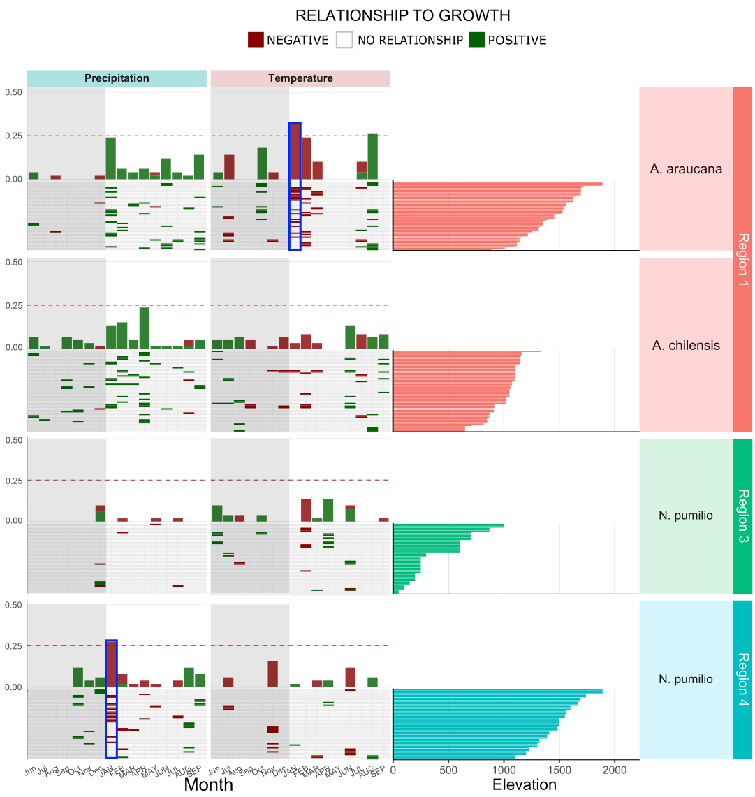
Figure 13. Heat map showing the responses of each chronology to climate. Chronologies were ordered by elevation from high to low which can be seen in details in right-hand side of the panel. Above each heat map the frequency plot demonstrating the sum of results from all chronologies in group, i.e. fragmented bars in the bottom add up to form the full bar in the top. The blue rectangles evidences the increase in response frequency at higher elevations.
At last, we investigated if the size of the response increases with the elevation. We thought that if it becomes more frequent, it is possible that it is due to increase in effect. To investigate that we tested the response coefficients as a function of elevation. We performed this analysis on the variables that were deemed to significantly affect species growth.
The regression analysis showed a negative correlation to elevation demonstrating that the size of the response is influenced by the elevation (Figure 14). This is likely due to the drier conditions that are generally found at higher elevations but it provides evidence that species at higher elevations are most likely to be more vulnerable to changing conditions.
The regression analysis showed a negative correlation to elevation demonstrating that the size of the response is influenced by the elevation (Figure 14). This is likely due to the drier conditions that are generally found at higher elevations but it provides evidence that species at higher elevations are most likely to be more vulnerable to changing conditions.
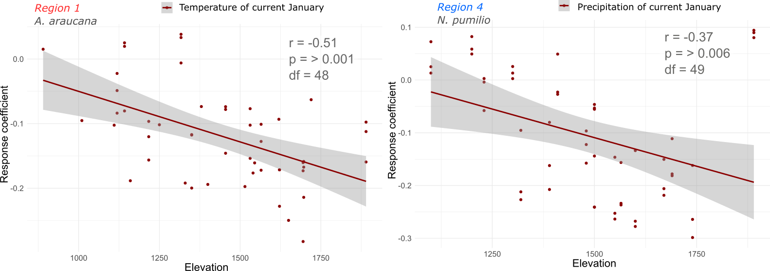
Figure 14. Correlations between response coefficient and elevation for A. araucana (region 1) and N. pumilio (region 4). Significant correlations (p = >0.05) demonstrates that the response effect increases at higher elevations.
Our models here are somewhat in accordance with the map from Boisvenue and Running (2006) that says that a mix of water and temperature are limiting tree growth. However, it is evidenced a fair amount of variation due to inter and intra specific responses. Since average temperature is predicted to increase and average precipitation predicted to decrease (Magrin et al. 2014), the species mentioned on figure 12 are likely to become vulnerable to extended and more intense drought events. In turn, this may increase the probability of dieback to occur in this region (Allen et al. 2010). Although some patterns were revealed regarding the factors affecting tree growth bringing us closer to understand the mortality threshold as described by Allen et al. (2010), there is still research needed to point at what temperature, precipitation and elevations the chance of great diebacks to occur increase above historical/natural values.
